'''
서울시 각 구별 CCTV 수를 파악하고,
인구대비 CCTV 비율을 파악해서 순위 비교
서울시 각 구별 CCTV 수 : 01. CCTV_in_Seoul.csv
서울시 인구 현황 : 01. population_in_Seoul.xls
'''
import pandas as pd
CCTV_Seoul = pd.read_csv("01. CCTV_in_Seoul.csv", encoding='utf-8')
CCTV_Seoul.head()
CCTV_Seoul.info()
# 기관명 컬럼의 이름을 '구별' 컬럼으로 변경하기
CCTV_Seoul.rename(columns={'기관명':'구별'},inplace=True)
CCTV_Seoul.head()
# 첫번째 컬럼의 이름을 '구별'로 컬럼명을 변경하기
CCTV_Seoul.rename(columns={CCTV_Seoul.columns[0]:'구별'},inplace=True)
CCTV_Seoul.head()
# 서울시 인구 현황 읽기
pop_Seoul = pd.read_excel("01. population_in_Seoul.xls")
pop_Seoul.head()
# 엑셀파일의 해더 부분 복잡하여 3번째 행을 해더로 처리 필요
# 또한 열도 선택하여 저장 필요
pop_Seoul = pd.read_excel("01. population_in_Seoul.xls", header=2, usecols='B, D, G, J, N')
pop_Seoul.head()
# 컬럼명도 수정 필요
# 첫번째 : 구별, 두번째 : 인구수, 세번째 : 한국인, 네번째 : 외국인, 다섯번째 : 고령자
pop_Seoul.rename(columns={pop_Seoul.columns[0]:'구별',
pop_Seoul.columns[1]:'인구수',
pop_Seoul.columns[2]:'한국인',
pop_Seoul.columns[3]:'외국인',
pop_Seoul.columns[4]:'고령자'},inplace=True)
pop_Seoul.head()
# 첫번째(합계) 행 제거 필요
pop_Seoul.drop([0],inplace=True)
pop_Seoul.head()
# 최근 증가율 컬럼 추가
# 2014년부터 2016년까지 최근 3년간 CCTV수의 합과
# 2013년 이전 CCTV수로 나눠 최근 3년간 CCTV 증가율 계산
# 최근 증가율이 많은 5개로 구를 조회
CCTV_Seoul.head()
CCTV_Seoul["최근증가율"] = ((CCTV_Seoul["2014년"] + CCTV_Seoul["2015년"] + CCTV_Seoul["2016년"]) / CCTV_Seoul["2013년도 이전"]) * 100
CCTV_Seoul.sort_values(by='최근증가율',ascending=False).head(5)
# 외국인 비율, 고령자 비율 컬럼 추가하기
pop_Seoul['외국인비율'] = pop_Seoul['외국인'] / pop_Seoul['인구수'] * 100
pop_Seoul['고령자비율'] = pop_Seoul['고령자'] / pop_Seoul['인구수'] * 100
pop_Seoul.head()
# 외국인 비율 높은 구 5개
pop_Seoul.sort_values(by='외국인비율',ascending=False).head(5)
'''
CCTV 데이터와 인구 데이터 합치고 분석하기
'''
CCTV_Seoul.head()
pop_Seoul.head()
data_result = pd.merge(CCTV_Seoul, pop_Seoul, on = '구별')
data_result.head()
'''
2013년도 이전, 2014년, 2015년, 2016년 컬럼 제거하기.
'''
del data_result["2013년도 이전"]
del data_result["2014년"]
del data_result["2015년"]
del data_result["2016년"]
data_result.head()
# 인덱스를 구별 컬럼으로 변경하기. 구별 컬럼을 인덱스로 만들기
data_result.set_index('구별',inplace=True)
data_result.head()
# 상관계수
data_result.corr(method='pearson')
# 고령자 비율과 소계 두개의 피쳐간의 상관계수 구하기
import numpy as np
np.corrcoef(data_result["고령자비율"],data_result["소계"])
# 외국인 비율과 소계 두개의 피처간의 상관계수 구하기
np.corrcoef(data_result["외국인비율"],data_result["소계"])
# 인구수와 소계 두개 피처간의 상관계수 구하기
np.corrcoef(data_result["인구수"],data_result["소계"])
# matplot을 이용한 그래프 작성하기
# CCTV 갯수를 막대그래프로 작성하기
import matplotlib.pyplot as plt
from matplotlib import font_manager, rc
plt.figure()
data_result['소계'].plot(kind='barh',grid=True,figsize=(10,10))
plt.show()
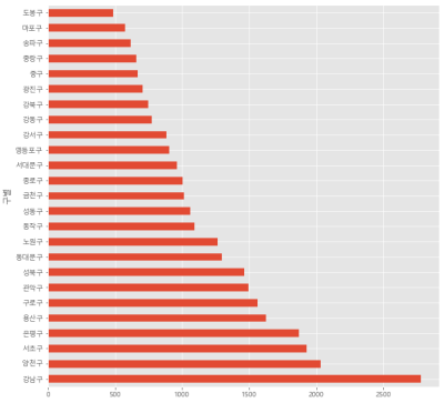
# 그래프를 소계의 내림차순으로 수평막대 그래프 작성
data_result.sort_values(by="소계",ascending=False,inplace=True)
data_result['소계'].plot(kind='barh',grid=True,figsize=(10,10))
plt.show()
'''
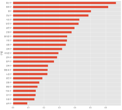
인구수 대비 CCTV 비율 컬럼 추가하기
소계 / 인구수
'''
data_result["CCTV비율"] = data_result["소계"]/data_result["인구수"]*100
data_result["CCTV비율"].sort_values().plot(kind='barh',grid=True,figsize=(10,10))
plt.show()
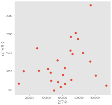
# 산점도 그리기
# 인구수와 소계 산점도 작성하기
plt.figure(figsize=(6,6))
plt.scatter(data_result["인구수"], data_result["소계"], s=50)
plt.xlabel("인구수")
plt.ylabel("CCTV갯수")
plt.grid()
plt.show()
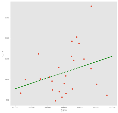
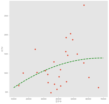
# 인구수와 소계 산점도, 회귀선 작성하기
# fp1 : 최소제곱법 이용한 상수값
# 1 : 직선
fp1 = np.polyfit(data_result['인구수'], data_result['소계'],1)
f1 = np.poly1d(fp1)
fx = np.linspace(100000,700000,100) #10만~70만 100개 간격
plt.figure(figsize=(10,10))
plt.scatter(data_result['인구수'],data_result["소계"],s=50)
plt.plot(fx,f1(fx),ls='dashed',lw=3,color='g') #ls는 줄의 종류 #lw는 줄 굵기
plt.xlabel('인구수')
plt.ylabel('CCTV')
plt.grid()
plt.show()
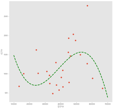
# 인구수와 소계 산점도, 회귀선 작성하기
# fp1 : 최소제곱법 이용한 상수값
# 2 : 2차원(곡선)
fp1 = np.polyfit(data_result['인구수'], data_result['소계'],2)
f1 = np.poly1d(fp1)
fx = np.linspace(100000,700000,100) #10만~70만 100개 간격
plt.figure(figsize=(10,10))
plt.scatter(data_result['인구수'],data_result["소계"],s=50)
plt.plot(fx,f1(fx),ls='dashed',lw=3,color='g') #ls는 줄의 종류 #lw는 줄 굵기
plt.xlabel('인구수')
plt.ylabel('CCTV')
plt.grid()
plt.show()
# 인구수와 소계 산점도, 회귀선 작성하기
# fp1 : 최소제곱법 이용한 상수값
# 3 : 3차원(곡선)
fp1 = np.polyfit(data_result['인구수'], data_result['소계'],3)
f1 = np.poly1d(fp1)
fx = np.linspace(100000,700000,100) #10만~70만 100개 간격
plt.figure(figsize=(10,10))
plt.scatter(data_result['인구수'],data_result["소계"],s=50)
plt.plot(fx,f1(fx),ls='dashed',lw=3,color='g') #ls는 줄의 종류 #lw는 줄 굵기
plt.xlabel('인구수')
plt.ylabel('CCTV')
plt.grid()
plt.show()
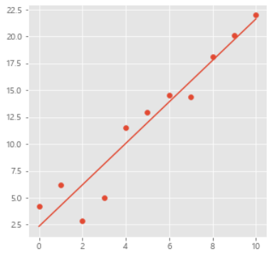
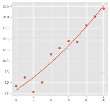
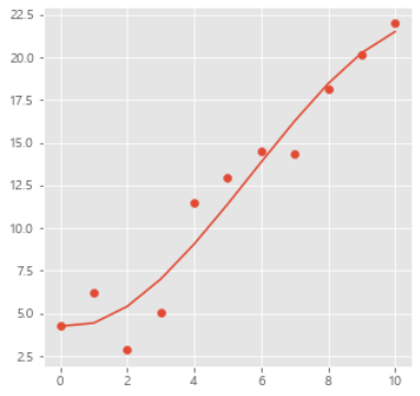
# polyfit 상수를 이용한 회귀선 예제
import numpy as np
x = np.array([0.,1.,2.,3.,4.,5.,6.,7.,8.,9.,10.])
y = np.array([4.23620563,6.18696492,2.83930821,5.00923197,11.51299327,12.91581993,14.51838241,14.348811875,18.13566499,20.1408104,21.9872241])
fit1 = np.polyfit(x,y,1)
fit2 = np.polyfit(x,y,2)
fit3 = np.polyfit(x,y,3)
print(fit1) #[1.92858267 2.34176099]
print(fit2) #[0.05915417 1.33704093 3.2290736 ]
print(fit3) #[-0.02808822 0.48047747 -0.26960522 4.2402495 ]
'''
polyfit : 각 차원의 최소 거리에 맞는 기울기와 절편값을 제공한다.
직선 : 1차원 : y = ax+b / a:기울기, b:절펀
곡선 : 2차원 : y = ax**2 + bx + c / a: 기울기, c : 절편
곡선 : 3차원 = y = ax***3 + bx**2 + bx + d / d: 절편
'''
num = len(x)
for i in range(num):
fit1= 1.9285826*x + 2.34176099
fit2 = 0.05915417*x**2 + 1.33704093*x + 3.2290736
fit3 = -0.02808822*x**3 + 0.48047747*x**2 - 0.26960522*x + 4.2402495
print(fit1)
# x,y 산점도와 회귀선을 출력하기
plt.figure(figsize=(5,5))
plt.scatter(x,y)
plt.plot(x,fit1)
plt.show()
plt.figure(figsize=(5,5))
plt.scatter(x,y)
plt.plot(x,fit2)
plt.show()
plt.figure(figsize=(5,5))
plt.scatter(x,y)
plt.plot(x,fit3)
plt.show()
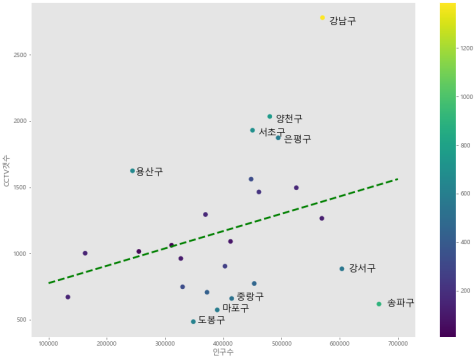
# 산점도 + 회귀선. 산점도에 점의 색상을 회귀선과의 거리 표시
# 회귀선을 위한 상수
fp1 = np.polyfit(data_result['인구수'], data_result['소계'],1)
# fp1 상수 값을 이용해서 회귀선의 y 값을 계산하기 위한 함수 설정
f1 = np.poly1d(fp1)
fx = np.linspace(100000,700000,100) # x축의 값 10만~70만까지 100등분
# f1(data_result['인구수']) : 인구수에 맞는 회귀선의 y값
# data_result['소계'] 와의 절대값 차이
data_result['오차'] = np.abs(data_result['소계'] - f1(data_result['인구수']))
data_result.head()
df_sort = data_result.sort_values(by='오차', ascending=False)
# c = data_result['오차'] : 점의 색상을 오차에 맞도록 설정
plt.figure(figsize=(14,10))
plt.scatter(data_result['인구수'],data_result['소계'],c=data_result['오차'],s=50)
plt.plot(fx,f1(fx),ls='dashed',lw=3,color='g')
# 점에 해당하는 구의 이름 오차가 많은 구 10개 정보를 표시하기
for n in range(10):
plt.text(df_sort['인구수'][n]*1.02, df_sort['소계'][n]*0.98,df_sort.index[n],fontsize=15)
plt.rc('font',family="Malgun Gothic")
plt.xlabel('인구수')
plt.ylabel('CCTV갯수')
plt.colorbar()
plt.grid()
plt.show()
'Python' 카테고리의 다른 글
| Python - KNN(K-Nearest-Neighbors) (0) | 2021.07.16 |
|---|---|
| Python - 회귀분석(Regression) (0) | 2021.07.15 |
| Python - 웹크롤링 후 텍스트 마이닝 (seleium) (0) | 2021.07.13 |
| Python - 웹크롤링 (BeautifulSoup/ Selenium) (0) | 2021.07.06 |
| Python - 변수저장, 데이터프레임 필터(조회기능), 데이터프레임 병합 (0) | 2021.07.05 |


